


P-computing system compatible with CIM and its core artificial tunable p-bit
Our p-computing platform is built upon the architecture of a discrete Hopfield Neural Network (DHNN)7,26, as shown in Fig. 2a. DHNN is a single-layer, recurrent neural network characterized by self-feedback and interconnections. This architecture performs optimization by minimizing the following energy function:
$$E=-\frac{1}{2}{\sum }_{i,j}{J}_{{ij}}{x}_{i}{x}_{j}-{\sum }_{i}{h}_{i}{x}_{i}$$
(1)
where Jij represents the interconnection matrix between p-bits, hi denotes the local bias of the i-th p-bit, and xi is the instantaneous state of the p-bit, which takes binary values 0 or 1.

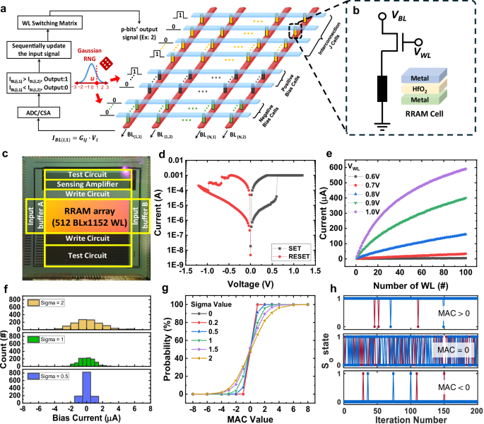
a Schematic of the compute-in-memory (CIM) hardware mapping under the discrete Hopfield Neural Network (DHNN) architecture, in which interconnection values are encoded using pairs of RRAM cells. A p-bit with tunable stochasticity is activated by different numbers of cells in the bias region. b 1T1R structure of the DHNN hardware, which needs to be used in conjunction with subsequent Gaussian random number generator (GRNG) and comparator circuits. c Photograph of the p-computing chip integrating the 1T1R RRAM array with the 180-nm CMOS technology. d Characteristics of switching curves of the standalone RRAM cell. e Experimentally measured cumulated bit line (BL) current, namely the multiply-accumulate (MAC) output by activating different numbers of word lines (WLs) at different WL voltages. f Bias current distributions controlled by the sigma value of the GRNG at standard deviation σ = 0.5, 1, and 2. g A series of sigmoidal probability curves of the artificial tunable p-bit (probability of output being 1) under different sigma values ranging from 0 to 2. h Time snapshots of the output states for three different inputs (MAC = +4, 0, and −4, respectively) observed experimentally (solid blue line) and by simulation (solid red line) at σ = 2.
However, a standard DHNN encounters challenges when solving complex COPs, as it is prone to getting trapped in local energy minima, thereby limiting the exploration of global optimal solutions. To address this issue, we introduced an in-RRAM bias with GRNG into the system, which adjusts the stochasticity of p-bits during the state update process (implementation details are provided in Supplementary Note 1). This enhanced randomness increases the likelihood of escaping local minima, thereby improving the system’s capability to explore the solution space globally. During the iterative process for solving the molecular docking problem, the p-bits’ states are updated according to the following rules:
$${\sum }_{j}{J}_{{ij}}{x}_{j}+{h}_{i}={s}_{{{\rm{in}}}},\left\{\begin{array}{c}{s}_{{{\rm{in}}}}\ge u,{x}_{i}^{{{\rm{new}}}}=1\\ {s}_{{{\rm{in}}}} < u,{x}_{i}^{{{\rm{new}}}}=0\end{array}\right.$$
(2)
where sin represents the net input to the i-th p-bit, and u is the dynamic threshold value provided by the GRNG, which is taken as an integer. A detailed theoretical derivation of the GRNG-based p-bit mechanism is provided in the “Methods” section. On the other hand, conventional DHNN employs a sequential state update scheme to ensure stable convergence. To fully exploit the inherent parallelism of RRAM-based architecture, a parallel evaluation scheme can be adopted. In this approach, all output states are evaluated simultaneously to identify valid update candidates, from which a single bit is randomly selected for state updating.
To implement this p-computing framework in hardware, we adopted HfO₂-based RRAM as the core device for this DHNN architecture. RRAM offers high density, low power consumption, and non-volatility, making it an ideal choice for hardware-level p-bit networks. In this system, the RRAM chip not only serves as a storage element but is also integrated closely with peripheral sensing circuit to generate tunable stochastic output signals, enabling the core functionality of p-bits. Figure 2b illustrates the 1T1R array structure of the p-computing chip integrating the RRAM array with the 180-nm CMOS technology in Fig. 2c, where “R” represents the HfO₂-based RRAM cell. This device consists of a top metal electrode, an HfO₂ resistive switching layer, and a bottom metal electrode. Its conductance state is modulated by controlling the bit line (BL) voltage VBL and word-line (WL) voltage VWL. When an external voltage is applied between the electrodes, oxygen vacancies in the HfO₂ layer are activated, leading to the formation or rupture of conductive filaments and enabling reversible switching between the high-resistance state (HRS) and low-resistance state (LRS). This bipolar switching behavior is clearly demonstrated in Fig. 2d, which shows the current-voltage characteristics of the RRAM cell. Figure 2e presents the relationship between the cumulative current on the BL and the number of WLs under different VWL. At lower VWL values, e.g., 0.6 V and 0.7 V, the BL current shows a good linear relationship with the number of WLs. However, at higher VWL, the cumulative current increases more rapidly, deviating from the linear trend due to the IR drop issue56. This observation suggests that appropriately reducing the WL voltage helps preserve the linearity of BL current, thereby improving the consistency and reliability of array’s performance (details in Supplementary Note 2). Furthermore, the 1T1R array architecture inherently eliminates the problem of sneak path currents. Since each RRAM cell is controlled by its dedicated access transistor, current flow is strictly confined to the selected cell during read and write operations. This structural isolation prevents unintended current leakage through unselected cells, which is a well-known issue in selector-less crossbar (1R) arrays. As a result, our design guarantees reliable readout and switching behavior without the interference of sneak currents, ensuring consistent device performance across the array. More detailed electrical characteristics of the core cell are provided in Supplementary Note 3.
Figure 2f highlights the key mechanism for this tunable p-bit functionality achieved through in-array random bias. This method leverages a GRNG to control the number of activated WLs in the bias region, dynamically modulating the distribution of bias current. Device-to-device and cycle-to-cycle variations are minimized through RRAM duplication and read-averaging techniques (see Supplementary Note 4). The standard deviation σ of the bias current distribution can be flexibly adjusted for implementing the DSA algorithm. When σ is small, the bias current distribution is narrow and sharply peaked. As σ increases, the distribution broadens, and randomness is significantly enhanced. This high-tunability bias current control mechanism forms the foundation for the tunable p-bit functionality. It stands in sharp contrast to conventional RRAM-based true random number generators, which generate uniformly distributed random bits for general-purpose cryptographic or stochastic computing57,58. Instead, our system employs a controllable Gaussian-distributed threshold for p-bit activation. Furthermore, as shown in Fig. 2g, after the comparison process, the probability of a p-bit outputting a value of 1 under different σ values exhibits a typical sigmoidal (S-shaped) stochastic characteristic as a function of the MAC input. The range and slope of the probability response vary with σ, enabling deliberate adjustment steepness of the sigmoid curve to optimize the state update process. Figure 2h demonstrates the real-time fluctuation behavior of a p-bit under σ = 2. When the MAC value is positive, the p-bit output state is predominantly 1, with occasional state transitions, indicating high determinism toward the high state. When the MAC value is zero, the p-bit output oscillates randomly, with nearly equal proportions of 0 and 1, resembling a random number generator with a uniform binary distribution. For negative MAC values, the p-bit output stays at 0 for most cycles, with infrequent transitions to 1.
Translation of molecular docking to maximum weighted clique problem
Molecular docking is a complex computational problem that is central to structure-based drug design. It involves identifying the binding interactions between pharmacophore points (PPs) on ligands and receptor proteins, which are critical for determining biological or pharmacological interactions. PPs, characterized by properties such as electrostatic characteristics, hydrophobicity, and hydrogen bond donor/acceptor capabilities, play a crucial role in molecular recognition and binding affinity. In this study, we focus on the LolCDE protein complex, a key component of Gram-negative bacteria, which works in conjunction with the periplasmic chaperone LolA to transport lipoproteins from the inner membrane to the outer membrane59. This process is essential for bacterial physiology and pathogenicity, as lipoproteins play crucial roles in cell wall synthesis, bacteria-host interactions, and stress signal transmission60. Disrupting this transport process provides a promising strategy for developing antibacterial drugs targeting lipoprotein transport and potentially addresses the growing threat of drug-resistant Gram-negative bacteria. A recent structural biology study utilized high-resolution three-dimensional structures to resolve the ternary complex formed by the LolCDE complex with lipoproteins and the LolA protein, which provided a structural basis for an in-depth understanding of the molecular mechanism of lipoprotein transport61.
As illustrated in Fig. 3a, we identified 6 PPs on the lipoprotein and 7 PPs on the LolA-LolCDE protein complex. For the lipoprotein, these points were classified based on their chemical properties into hydrophobic (hp1–hp5) and hydrogen bond acceptor (ha1) categories. Correspondingly, the PPs on the protein complex were categorized as hydrophobic (HP1–HP5) and hydrogen bond donor (HD1 and HD2). These PPs theoretically give rise to 42 potential ligand-receptor pharmacophore binding pair modes, where each pair involves one PP from the ligand and one from the receptor protein, as depicted in Fig. 3b. Subsequently, an undirected, fully connected graph with 42 vertices was constructed, where each potential pharmacophore binding pair corresponds to a vertex. However, not all pharmacophore binding pairs can coexist in the spatial structure. Therefore, we performed a spatial compatibility check by quantifying the spatial relationship between these PPs on their respective 3D structure based on Euclidean distances (Supplementary Fig. 2). Briefly, two binding pairs are deemed compatible only if the distance difference between the PPs satisfies specific criteria (see details in “Methods”). The adjacency matrix shown in Fig. 3c captures the coexistence of these 42 vertices after the compatibility check, where black squares indicate compatibility (spatial coexistence of two vertices) and white squares representing incompatibility. Finally, a binding interaction graph (BIG), denoted as GB = (V, E) was generated, as shown in Fig. 3d. In this graph, each edge Eij∈E indicates that the binding pair represented by vertices Vi and Vj are spatially compatible. Additionally, each vertex Vi is assigned a weight wi. It represents the knowledge-based binding potential of the corresponding binding pair derived from the PDBbind dataset62,63,64, as shown in Table 1 (the weight of each vertex is detailed in Supplementary Table 1). These weights reflect the relative strength of interactions and the contribution of each binding pair to the overall molecular binding affinity. The formation of cliques within the structure of GB implies a group of pharmacophore binding pairs that are mutually compatible and collectively define a feasible docking conformation. Among these cliques, the one with the maximum weight is referred to as the maximum weighted clique (MWC), which corresponds to the most energetically favorable and stable docking conformation. This clique maximizes the total binding potential energy while satisfying the spatial compatibility constraints.

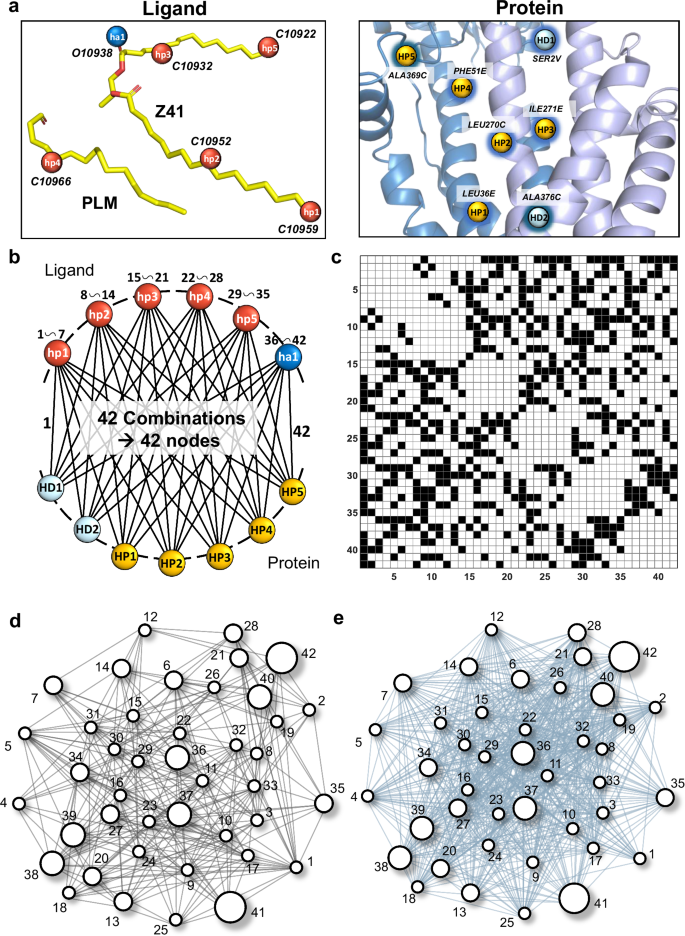
a Identified 6 pharmacophore points (PPs) on the lipoprotein (left) with the Protein Data Bank (PDB) ID of 7ARM: C10959 (hp1), C10952 (hp2), C10932 (hp3), C10966 (hp4), C10922 (hp5), and O10938 (ha1), located on the PLM and Z41 branches. Identified 7 PPs on the LolCDE-LolA complex (right): HP1 (C3214, residue LEU36E), HP2 (C2057, LEU270C), HP3 (C5034, ILE271E), HP4 (C3313, PHE51E), HP5 (C2758, ALA369C), HD1 (O9421, SER2V), and HD2 (O2805, ALA376C). b Pharmacophore binding pairs between the ligand and the protein. Each line represents a potential pharmacophore binding pair and is sequentially named, starting from hp1-HP1 (node 1),…, hp1-HD2 (node 7) to ha1-HD2 (node 42). c Adjacency matrix after the spatial compatible check. d Binding interaction graph GB of this docking problem. e Self-complementary graph of GB, where vertices with different weights are shown in different sizes.
To date, the molecular docking problem has been transformed into a MWCP, enabling us to shift focus from the complex, high-dimensional conformational space of ligand-receptor interactions to a well-defined mathematical problem in graph theory. To solve this efficiently, we further reformulate the MWCP into a QUBO problem65, expressed as:
$$F\left(X\right)={\sum }_{i=1}^{N}{w}_{i}{x}_{i}+\frac{1}{2}{\sum }_{i,j}^{N}{J}_{{ij}({G}_{{{\rm{B}}}})}{x}_{i}{x}_{j}.$$
(3)
where the first term represents the total weight of the vertices included in the clique, while the second term accounts for the connectivity amongst the vertices. Matrix Jij(GB) represents the interconnectivity of vertex Vi and vertex Vj in the BIG. Specifically, Jij(GB) = 1, if the two vertices are connected by an edge, the Jij(GB) = 0 otherwise.
The maximization of this quadratic function returns a subset of vertices that form a clique while maximizing the total weight. To align with the principle and the architecture of our p-computer, we refined the problem formulation. Equation (3) was reformulated to represent the maximization of the sum of vertex weights in an energy minimization form and penalty terms were introduced to enforce connectivity constraints within the GB:
$$E\left(X\right)=-A\cdot {\sum }_{i=1}^{N}{w}_{i}{x}_{i}+\frac{P}{2}\cdot {\sum }_{i,j}^{N}{J}_{{ij}(\overline{{G}_{{{\rm{B}}}}})}{x}_{i}{x}_{j}.$$
(4)
where the first term minimizes the energy expression to maximize the total weight of selected vertices, while the second term introduces a penalty factor P for pairs of adjacent vertices in the self-complementary graph \(\overline{{G}_{{{\rm{B}}}}}\) shown as in Fig. 3e. The relationship of interconnectivity of these two graphs is \({J}_{{ij}(\overline{{G}_{{{\rm{B}}}}})}=1-{I}_{n\times n}-{J}_{{ij}\left({G}_{{{\rm{B}}}}\right)}\), where \({I}_{n\times n}\) is an identity matrix and n is the number of vertices in GB.
Here, the parameter A serves as a balance control factor to regulate the influence of the weight term on the total energy. A larger value of A causes the weight term to dominate the energy minimization process; however, this dominance can weaken spatial constraint conditions, potentially resulting in solutions that fail to conform to clique structures. Conversely, increasing P strengthens the spatial constraints among variables in BIG, ensuring that the candidate solutions satisfy the compatibility requirements. However, an excessively large P significantly increases the hardware overhead when mapping Jij matrix to the RRAM chip. To address this issue, in the hardware implementation, we set A and P to 10 and 18, respectively, to strike a balance between these two terms (see Supplementary Note 5). This configuration effectively guides our hardware-based p-computing system toward efficient and accurate energy optimization within the solution space.
Experimental demonstration of a 42-node molecular docking
To systematically evaluate the performance of our RRAM-based p-computer in real molecular docking scenarios, framed as a MWCP, we modulated the stochasticity of the system by varying the standard deviation σ of the GRNG. Figure 4 illustrates the energy fluctuation profiles during iterations, the solution distributions, and the final predicted MWC across 100 independent experimental trials for each σ setting. Under constant stochasticity, the probabilistic state update of each p-bit follows the Gaussian-threshold rule introduced in “Methods”. The output probability is given by the Gaussian CDF, which closely approximates the sigmoid function commonly used in Boltzmann or Ising machines. Therefore, the steady-state probability distribution of the p-computer can be approximately expected from the Boltzmann law:
$$P\left(X\right)=\frac{\exp \left(-\frac{E\left(X\right)}{T}\right)}{{\sum }_{i,j}\exp \left(-\frac{E\left(X\right)}{T}\right)}$$
(5)
where T, referred to as the pseudo-temperature parameter in the context of p-computing, characterizes the system’s stochasticity. Consequently, the MWC corresponding to the ground state is expected to exhibit the highest probability. Following this principle, our p-computer identifies the most frequently occupied p-bit state configuration in each trial, represents it as a subgraph, and designates it as the trial’s output.

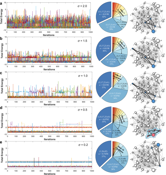
Energy dynamics during iterations (left), solution distributions (middle), and predicted multiply-accumulates (MWCs) (right) for varying levels of stochasticity: a σ = 2.0, b 1.5, c 1.0, d 0.5, and e 0.2, based on 100 independent trials per condition. Detailed experimental output subgraphs corresponding to these five stochasticity levels are provided in Supplementary Table 2 (σ = 2.0), Table 3 (σ = 1.5), Table 4 (σ = 1.0), Table 5 (σ = 0.5), and Table 6 (σ = 0.2).
Figure 4a shows that at the highest level of stochasticity (σ = 2.0), the system exhibited pronounced energy fluctuations, indicative of extensive and thorough exploration of the solution space. However, despite transiently reaching the theoretical ground state E = −8.702 at various points during the iterative process, which corresponds to an unidentified clique with a cumulative weight of 0.8702, the system ultimately failed to consistently occupy this optimal solution due to insufficient stability. Instead, the system predominantly produced lower-weight configurations, represented by (11, 17, 23, 41) and (5, 17, 23, 41), with cumulative weights of 0.8198 and occurrence frequencies of 32% and 29%, respectively.
Reducing σ to 1.5 (Fig. 4b) and 1.0 (Fig. 4c) mitigated the energy fluctuations, signaling a transition from broad exploration to localized oscillations around lower-energy configurations near −4 and −8. At these two stochasticity levels, the output subgraphs became more concentrated with the clique (5, 17, 23, 41), consistently emerging as the dominant solution in 36% and 37% of trials, respectively. However, despite the improved focus on low-energy configurations, like the clique with E = −8.702 ranked as the second most frequently observed output at σ = 1.0, the system still failed to reliably identify this optimal solution. As σ was further reduced to 0.5 (Fig. 4d), the system achieved a critical balance between exploration and identification. The considerably reduced stochasticity led to more confined energy fluctuations, shown as a distinct energy stratification at E = −5 and −8. Under this condition, the system occupied the ground state for the longest duration during the iterations, thus successfully identifying the theoretically optimal solution for the first time. The MWC (1, 9, 17, 25, 41) with a cumulative weight of 0.8702 emerged as the most frequent output clique, accounting for 35% of the trials. On the other hand, other candidate configurations, such as cliques (1, 26, 42) and (1, 21, 40), persisted, appearing in 15% and 12% of the outcomes, respectively. These lower-weight cliques represent local energy minima, where the system occasionally settles into during the evolvement process. Finally, at the lowest stochasticity level (σ = 0.2, Fig. 4e), the system exhibited minimal energy fluctuations. At this point, in addition to the GRNG, the contribution of device-to-device variations within the RRAM array becomes more prominent, but still in a low range. While this setting led to a more concentrated solution distribution, the system predominantly identified a non-optimal clique, (1, 26, 42), in 37% of trials, with the ground state occurring in only 26%. This outcome reveals a critical limitation of excessively low stochasticity, where restricted exploration leads the system to local optima, compromising its ability to achieve the ground state.
Figure 5a summarizes the simulation-based success probabilities of our RRAM–CIM p-computer in identifying the MWC across five stochasticity levels, comparing three scenarios: without annealing, with conventional SA, and with the DSA tailored for our CIM-based p-computer. The results show that while SA achieves moderate improvements at specific stochasticity levels (e.g., σ = 1.5), DSA exhibits enhancement across a broader range (σ = 0.5–2.0) and reaches higher success rates in certain cases. We attribute this advantage to DSA’s ability to mitigate premature convergence by maintaining higher levels of stochasticity during early iteration. This smooth annealing schedule facilitates a fast convergence to the global optimal solution. In contrast, the performance of SA is sensitive to its annealing schedule, with different decay strategies often leading to widely varying outcomes.

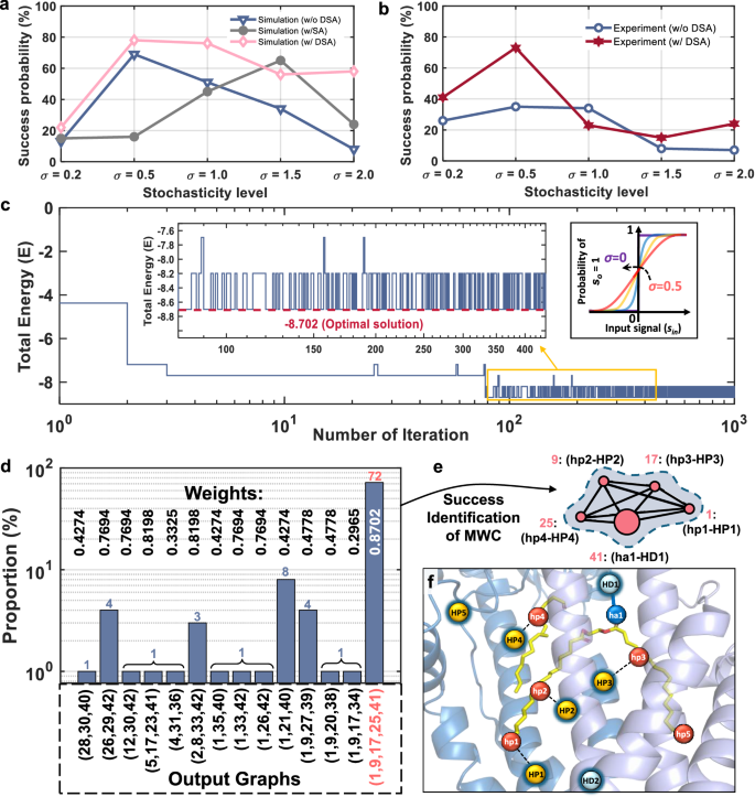
a Simulation-based success probability comparison of three scenarios: without any annealing schemes, including simulated annealing (SA) or dynamic slope annealing (DSA) (labeled as w/o DSA), with SA (labeled as w/ SA), and with DSA (labeled as w/ DSA). b Experiment-based success probability comparison with and without the application of DSA. For SA in simulations, a linear stochasticity decay schedule was adopted, while in the simulations and experiments using DSA, the Gaussian variance σ was linearly reduced from its initial value to zero. Each data point represents the average of 100 independent trials. c Dynamic evolution of the system’s energy during a complete 1000-iteration DSA process. Inset (left): detailed energy evolution at iterations 80 ~ 440. Inset (right): applied DSA schedule of σ decreased from 0.5 to 0. d Distribution of output solutions from 100 effective experimental trials. Detailed experimental output subgraphs are provided in Supplementary Table 7. e Graphical representation of the identified optimal maximum weighted clique (MWC), where the vertices and their corresponding exact binding pharmacophore point (PP) pairs are highlighted. f Cartoon representation of the predicted docking configuration between the ligand and the receptor protein.
Figure 5b compares the experimental success probabilities of identifying the MWC in 100 trials with the application of DSA approach against previous constant stochasticity settings. Without DSA, the success probability peaks at 35% for σ = 0.5. However, at lower stochasticity (σ = 0.2), restricted exploration leads to fluctuations among local energy minimums, while at higher stochasticity (σ = 1.5, 2.0), excessive noise inhibits the system’s ability to stabilize near optimal solutions. In contrast, the DSA strategy significantly improves success probability, achieving a peak at 72% by dynamically reducing σ from 0.5 to 0. This comparison underscores the importance of stochastic modulation in the p-computer, which enables the system to adaptively transition from global exploration to localized convergence. However, it does not always guarantee the improvement of MWC identification across all stochasticity levels, such as σ = 1.0. Factors such as device-to-device variations and inappropriate DSA schedule for a specific σ can limit the performance of this strategy. This underscores the critical importance of carefully tuning σ so that the stochasticity amplitude is of the same order as the deterministic signal range and of designing proper decay schedules to balance exploration and exploitation, as inappropriate values can either trap the system in local minima or introduce excessive randomness that hinders convergence. It should be emphasized that the primary objective of this study is not to claim algorithmic superiority of DSA over SA or other annealing schemes. Instead, our focus is to highlight the distinct hardware advantages of DSA, namely its compatibility with CIM-based p-computer, its ability to enable fully on-chip annealing at the p-bit hardware level natively, and its tighter integration with the GRNG-based p-computing framework.
A complete energy evolution of the system under the DSA application in a 1000-iteration process is shown in Fig. 5c. During the initial phase, the system exhibits significant energy fluctuations. This high level of stochasticity enables the system to effectively escape local minima and conduct a comprehensive exploration of the solution space. As DSA progresses and the stochasticity level gradually diminishes, the system transitions toward lower energy states, exhibiting increasingly stable oscillatory behavior. In the final stage of annealing, as σ approaches 0, the system’s energy stabilizes near the ground state (E = −8.702). However, due to the inherent device-to-device variations in the RRAM hardware, the system retains a small degree of randomness even when the GRNG’s σ is near 0. As shown in the left inset, this hardware-induced perturbation results in energy oscillations between global ground state and a sub-optimal state (E = −8.198), with the system exhibiting stronger preference for the ground state. Figure 5d presents the complete output subgraph distributions of the detailed 100 experimental trials conducted with DSA. Among the identified solutions, the clique (1, 9, 17, 25, 41), which corresponds to the ground state with a weight of 0.8702, emerged as the dominant outcome, achieving a success probability of 72%. In comparison, other candidate solutions, such as the cliques (1, 21, 40) with a weight of 0.4274 and (26, 29, 42) with a weight of 0.7694, occurred far less frequently, with success probabilities of 8% and 4%, respectively. Beyond the overall success probability, the effectiveness of DSA was further quantified by analyzing the first-hit time of the global optimum, defined as the iteration index at which the global optimum first appears within a trial. Under identical problem instance, the baseline system with constant stochasticity (σ = 0.5) reached the ground state after an average of 266.9 iterations, whereas DSA (σ decreasing from 0.5 to 0) achieved the same in only 63.6 iterations, corresponding to a ~ 4.2× acceleration. This quantitative evidence confirms that DSA both increases the success rate and substantially enhances convergence rate toward the global optimum. The MWC determined through this process is visualized in Fig. 5e. The resulting isolated subgraph highlights the vertices comprising the optimal solution, which directly corresponds to the matched PP binding pairs in this 42-node molecular docking problem. Specifically, vertices 1, 9, 17, 25, and 41 represent the binding PP pairs hp1-HP1, hp2-HP2, hp3-HP3, hp4-HP4, and ha1-HD1, respectively. Figure 5f provides the three-dimensional visualization of the predicted docking configuration between the lipoprotein and the LolCDE-LolA complex reconstructed from the identified MWC. This configuration includes four pairs of hydrophobic interactions and one hydrogen bond, collectively representing the most stable docking conformation with the highest binding affinity. Notably, the predicted binding mode closely aligns with the protein-ligand interactions analyzed using the Protein-Ligand Interaction Profiler (Supplementary Fig. 3)66,67, further validating the accuracy and reliability of our p-computer.
Overall, the 42-node docking experiment reveals how stochasticity fundamentally shapes the performance of our GRNG-based p-computer. High σ promotes broad search but prevents settling into the ground state, while very low σ amplifies RRAM device variations and leads to premature convergence. DSA alleviates this tension by exploiting stochasticity early and suppressing it later, thereby achieving both higher success probability and faster identification of the optimum. Together, these results demonstrate that the interplay between stochasticity, hardware non-idealities, and the evolving energy landscape necessitates a tightly integrated hardware–algorithm co-design to scale p-computing architectures toward large molecular docking and other COPs.
link